Report Design in R: Small Tweaks that Make a Big Difference

• Talk about how it was making multiple reports

Work With Other Tools

Make Ugly Reports

Make Beautiful Reports in R

* Results not guaranteed

Does Design Matter?

• Talk about how some devs don’t think it matters at all
• “I’m David and I think design matters because here’s what you can do with it”

Aesthetic Usability Effect

Users see aesthetically pleasing designs as more intuitive

Good Design Builds Trust

Putting effort into your charts shows respect for your audience, which means that they in turn are going to respect you and your findings.

But I’m Not a Designer!

But design is a skill that can be taught and R users already have many of the skills needed to do good design

I’m not a designer either

Good Design is Just a Few Small Tweaks

Framework for Good Design

• Do: Be consistent

• Don’t: Use defaults

What is a Report?

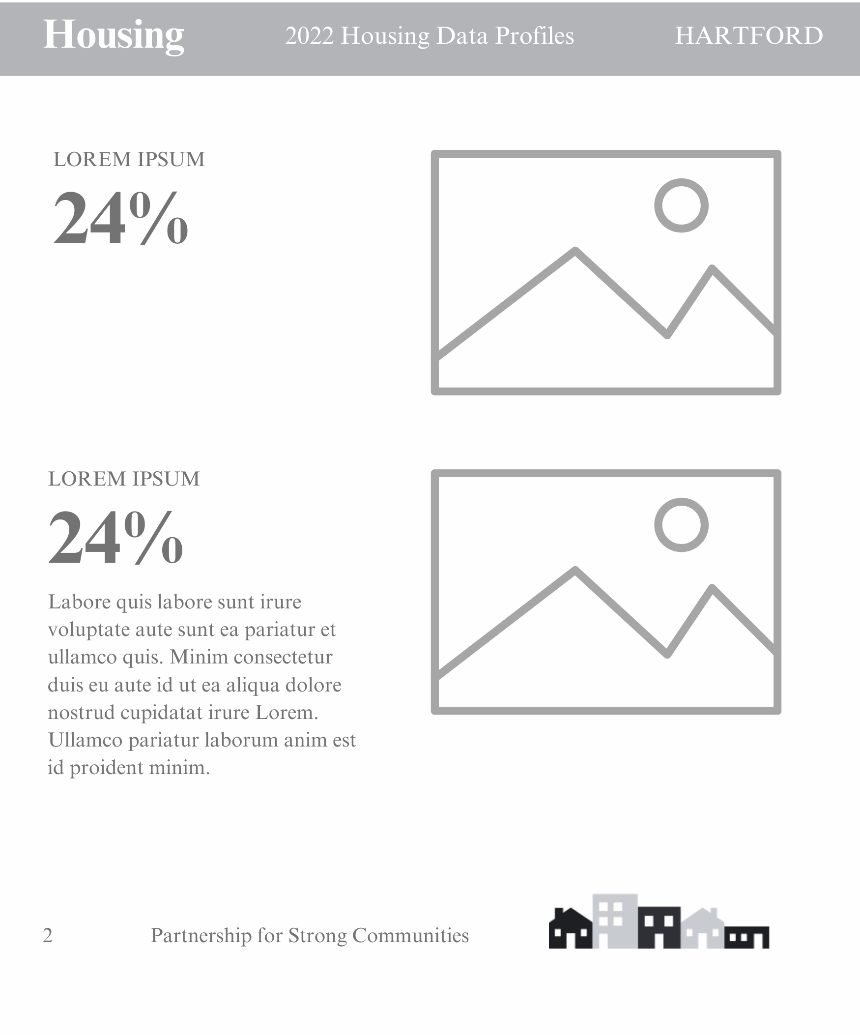
Create a Layout

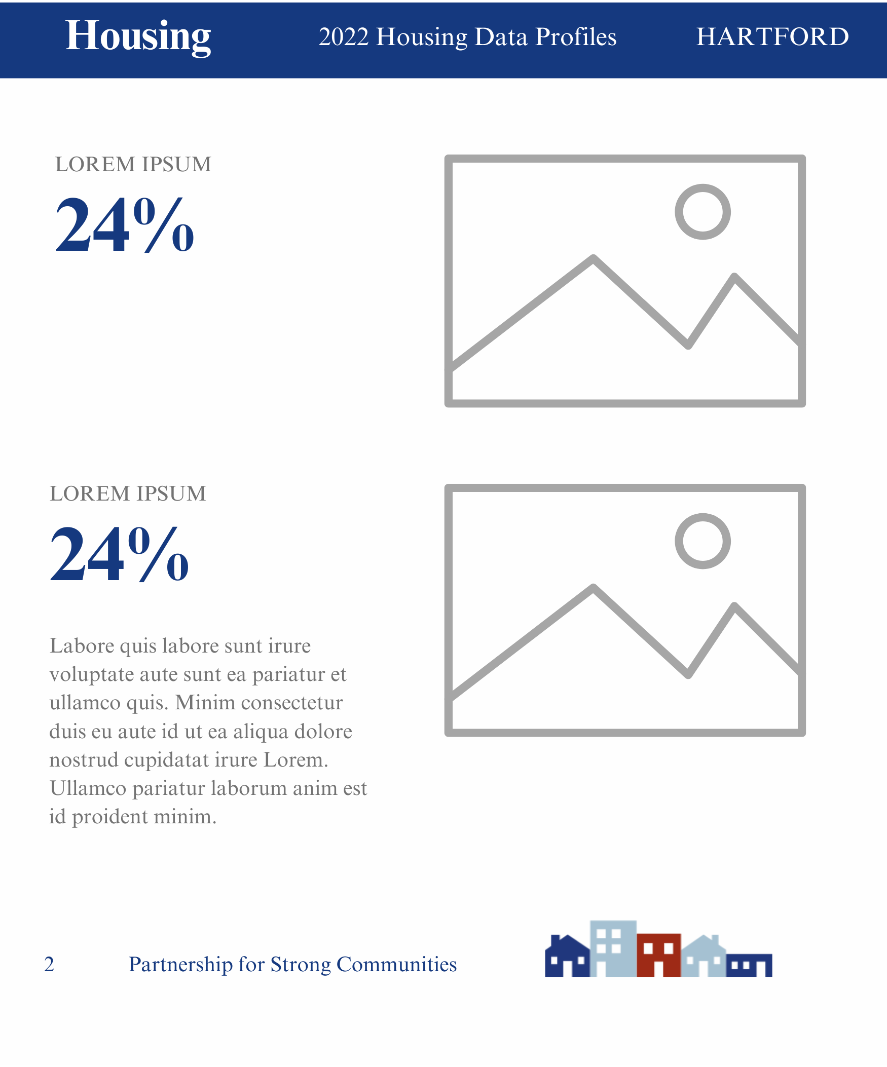
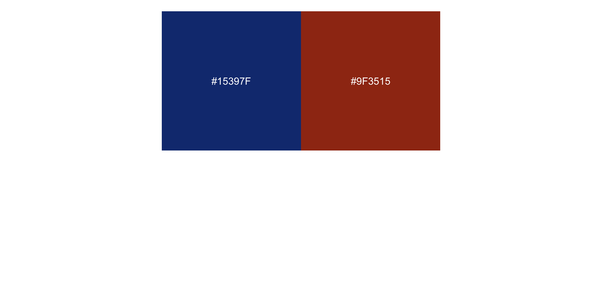
Add Brand Colors

Add Brand Fonts

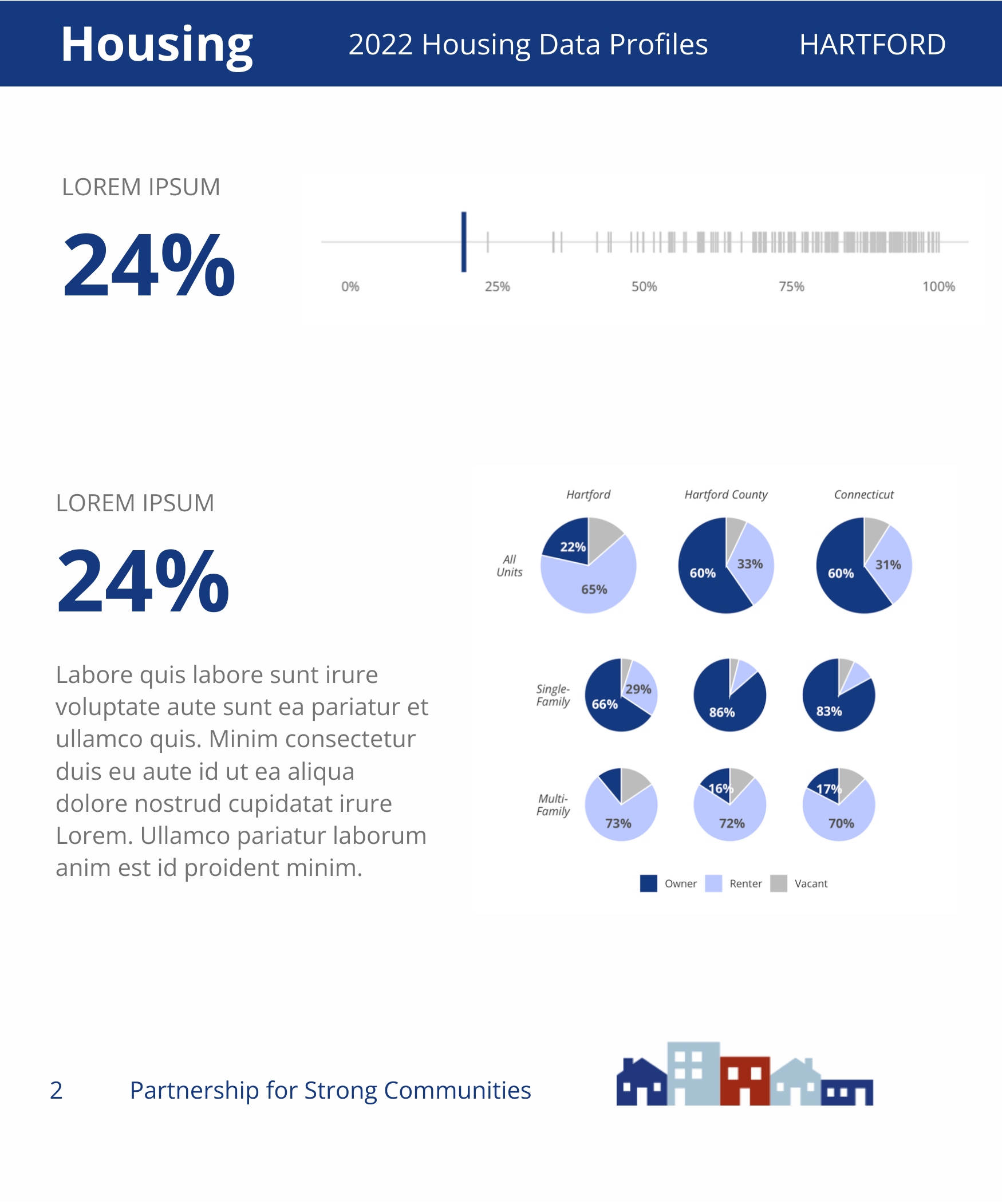
Add Plots

Identify Brand Colors

Identify Brand Fonts

Talk about how to identify fonts on websites

Create a Layout

typst

report.qmd

---
title: "Housing Data Profiles"

format: 
  typst:
    template-partials:
      - typst-show.typ
      - typst-template.typ

params:
  town: "Hartford"
---

# Introduction

Consequat occaecat mollit velit aliquip. Sunt Lorem ...

Mention that I will have link to slides and repo at end

report.qmd

---
title: "Housing Data Profiles"

format: 
  typst:
    template-partials:
      - typst-show.typ
      - typst-template.typ

params:
  town: "Hartford"
---

# Introduction

Consequat occaecat mollit velit aliquip. Sunt Lorem ...

typst-show.typ

#show: psc-report.with(
  $if(title)$
    title: "$title$",
  $endif$
  $if(params.town)$
    town: "$params.town$",
  $endif$
)

typst-show.typ

#show: psc-report.with(
  $if(title)$
    title: "$title$",
  $endif$
  $if(params.town)$
    town: "$params.town$",
  $endif$
)

typst-show.typ

#show: psc-report.with(
  $if(title)$
    title: "$title$",
  $endif$
  $if(params.town)$
    town: "$params.town$",
  $endif$
)

typst-template.typ

#let psc-report(
  title: "title",
  town: "town",
  body,
) = {

 set text()

 set page()

 body
}

typst-template.typ

#let psc-report(
  title: "title",
  town: "town",
  body,
) = {

 set text()

 set page()

 body
}

set text(
  font: "Open Sans",
  size: 12pt,
)

set page(
  "us-letter",
  margin: (left: 1in, 
           right: 1in, 
           top: 0.7in, 
           bottom: 1in)

background: 
  place(top, 
        rect(fill: rgb("15397F"), 
             width: 100%, 
             height: 0.5in))

header: align(
  horizon,
  grid(
    columns: (80%, 20%),
    align(left, 
          text(size: 20pt, 
               fill: white, 
               weight: "bold", 
               title)),
    align(right, 
          text(size: 12pt, 
               fill: white, 
               weight: "bold", 
               town)),
  ),
)

footer: align(
  grid(
    columns: (40%, 60%),
    align(horizon, 
          text(fill: rgb("15397F"), 
          size: 12pt, 
          counter(page).display("1"))),
    align(right, 
          image("assets/psclogo.svg", 
          height: 300%)),
  )

Use Functions to Make Your Plots Consistent

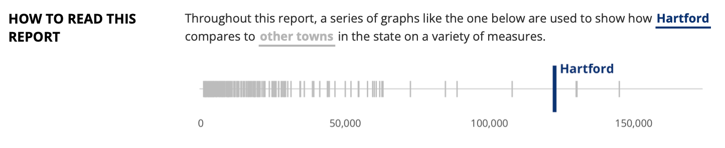
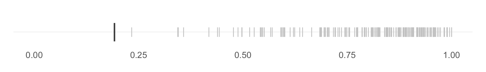
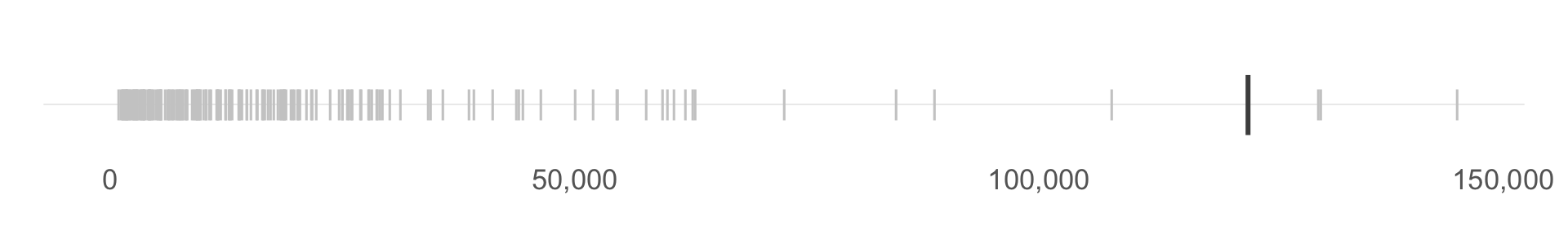
Comparison Plots

library(tidyverse)
library(scales)

single_family_homes

# A tibble: 169 × 2
    location         value
    <fct>            <dbl>
  1 Andover          0.897
  2 Ansonia          0.548
  3 Ashford          0.850
  4 Avon             0.844
  5 Barkhamsted      0.956
  6 Beacon Falls     0.717
  7 Berlin           0.807
  8 Bethany          0.958
  9 Bethel           0.746
 10 Bethlehem        0.944
 11 Bloomfield       0.704
 12 Bolton           0.966
 13 Bozrah           0.920
 14 Branford         0.684
 15 Bridgeport       0.345
 16 Bridgewater      0.982
 17 Bristol          0.591
 18 Brookfield       0.809
 19 Brooklyn         0.812
 20 Burlington       0.957
 21 Canaan           0.952
 22 Canterbury       0.925
 23 Canton           0.792
 24 Chaplin          0.901
 25 Cheshire         0.823
 26 Chester          0.786
 27 Clinton          0.811
 28 Colchester       0.786
 29 Colebrook        0.932
 30 Columbia         0.855
 31 Cornwall         0.961
 32 Coventry         0.933
 33 Cromwell         0.749
 34 Danbury          0.543
 35 Darien           0.909
 36 Deep River       0.721
 37 Derby            0.570
 38 Durham           0.970
 39 East Granby      0.773
 40 East Haddam      0.909
 41 East Hampton     0.872
 42 East Hartford    0.599
 43 East Haven       0.722
 44 East Lyme        0.814
 45 East Windsor     0.643
 46 Eastford         0.879
 47 Easton           1    
 48 Ellington        0.707
 49 Enfield          0.775
 50 Essex            0.791
 51 Fairfield        0.852
 52 Farmington       0.744
 53 Franklin         0.908
 54 Glastonbury      0.847
 55 Goshen           0.973
 56 Granby           0.934
 57 Greenwich        0.688
 58 Griswold         0.665
 59 Groton           0.542
 60 Guilford         0.889
 61 Haddam           0.928
 62 Hamden           0.601
 63 Hampton          0.884
 64 Hartford         0.192
 65 Hartland         0.962
 66 Harwinton        0.989
 67 Hebron           0.904
 68 Kent             0.861
 69 Killingly        0.624
 70 Killingworth     0.876
 71 Lebanon          0.950
 72 Ledyard          0.896
 73 Lisbon           0.890
 74 Litchfield       0.843
 75 Lyme             0.989
 76 Madison          0.930
 77 Manchester       0.551
 78 Mansfield        0.567
 79 Marlborough      0.923
 80 Meriden          0.546
 81 Middlebury       0.867
 82 Middlefield      0.906
 83 Middletown       0.478
 84 Milford          0.736
 85 Monroe           0.892
 86 Montville        0.825
 87 Morris           0.917
 88 Naugatuck        0.636
 89 New Britain      0.344
 90 New Canaan       0.822
 91 New Fairfield    0.983
 92 New Hartford     0.919
 93 New Haven        0.233
 94 New London       0.358
 95 New Milford      0.775
 96 Newington        0.749
 97 Newtown          0.930
 98 Norfolk          0.840
 99 North Branford   0.818
100 North Canaan     0.694
101 North Haven      0.843
102 North Stonington 0.960
103 Norwalk          0.527
104 Norwich          0.498
105 Old Lyme         0.885
106 Old Saybrook     0.873
107 Orange           0.924
108 Oxford           0.958
109 Plainfield       0.728
110 Plainville       0.613
111 Plymouth         0.754
112 Pomfret          0.856
113 Portland         0.840
114 Preston          0.948
115 Prospect         0.896
116 Putnam           0.516
117 Redding          0.867
118 Ridgefield       0.820
119 Rocky Hill       0.592
120 Roxbury          0.956
121 Salem            0.905
122 Salisbury        0.906
123 Scotland         0.917
124 Seymour          0.687
125 Sharon           0.917
126 Shelton          0.772
127 Sherman          0.990
128 Simsbury         0.791
129 Somers           0.935
130 South Windsor    0.824
131 Southbury        0.749
132 Southington      0.795
133 Sprague          0.696
134 Stafford         0.768
135 Stamford         0.443
136 Sterling         0.899
137 Stonington       0.732
138 Stratford        0.756
139 Suffield         0.876
140 Thomaston        0.698
141 Thompson         0.827
142 Tolland          0.942
143 Torrington       0.596
144 Trumbull         0.892
145 Union            1    
146 Vernon           0.488
147 Voluntown        0.846
148 Wallingford      0.686
149 Warren           0.990
150 Washington       0.891
151 Waterbury        0.419
152 Waterford        0.875
153 Watertown        0.796
154 West Hartford    0.702
155 West Haven       0.497
156 Westbrook        0.886
157 Weston           0.995
158 Westport         0.916
159 Wethersfield     0.801
160 Willington       0.621
161 Wilton           0.885
162 Winchester       0.596
163 Windham          0.439
164 Windsor          0.847
165 Windsor Locks    0.786
166 Wolcott          0.938
167 Woodbridge       0.927
168 Woodbury         0.828
169 Woodstock        0.895

comparison_plot <- function(
  df,
  highlight_town
) { }

comparison_plot <- function(df, highlight_town) {
  df |>
    ggplot(
      aes(
        x = value,
        y = 1
      )
    ) +
    ...
}

comparison_plot <- function(df, highlight_town) {
  df |>
    ggplot(
      aes(
        x = value,
        y = 1
      )
    ) +
    # Light gray lines for all towns
    geom_point(
      shape = 124,
      color = "gray80"
    ) +
    ...
}

comparison_plot <- function(df, highlight_town) {
  df |>
    ggplot(
      aes(
        x = value,
        y = 1
      )
    ) +
    # Light gray lines for all towns
    geom_point(
      shape = 124,
      color = "gray80"
    ) +
    # Line for town to highlight
    geom_point(
      data = df |> filter(location == highlight_town),
      shape = 124,
      color = "gray30"
    ) +
    ...
}

comparison_plot(
  df = single_family_homes,
  highlight_town = "Hartford"
)

comparison_plot <- function(df, highlight_town) {
  ggplot(
    aes(
      x = value,
      y = 1
    )
  ) +
    scale_x_continuous(
      labels = percent_format(accuracy = 1)
    ) +
    ...
}

comparison_plot <- function(
  df,
  highlight_town,
  value_type
) { }

comparison_plot <- function(df, highlight_town, value_type) {
  plot <-
    df |>
    ggplot() +
    ...

  if (value_type == "percent") {
    final_plot <- plot +
      scale_x_continuous(
        labels = percent_format(accuracy = 1)
      )
  }
}

comparison_plot <- function(df, highlight_town, value_type) {
  plot <-
    df |>
    ggplot() +
    ...

  if (value_type == "percent") {
    final_plot <- plot +
      scale_x_continuous(
        labels = percent_format(accuracy = 1)
      )
  }

  if (value_type == "number") {
    final_plot <- plot +
      scale_x_continuous(
        labels = comma_format(accuracy = 1)
      )
  }
}

comparison_plot(
  df = single_family_homes,
  highlight_town = "Hartford",
  value_type = "percent"
)

comparison_plot(
  df = total_population,
  highlight_town = "Hartford",
  value_type = "number"
)

Big Numbers

big_number_plot <- function(
  value,
  text
) { }

big_number_plot <- function(value, text) {
  ggplot() +
    # Add value
    geom_text(
      aes(
        x = 1,
        y = 1,
        label = value
      ),
      fontface = "bold",
      size = 20,
      hjust = 0
    ) +
    theme_void()
}

big_number_plot <- function(value, text) {
  ggplot() +
  # Add value
  ...
  # Add text
  geom_text(
    aes(
      x = 1,
      y = 2,
      label = str_to_upper(text)
    ),
    color = "gray70",
    size = 7,
    hjust = 0
  ) +
    theme_void()
}

big_number_plot <- function(value, text) {
  ggplot() +
  # Add value
  ...
  # Add text
  ...
  theme_void()
}

big_number_plot(
  value = "19%",
  text = "Single-Family Homes as\nPercent of All Homes"
)

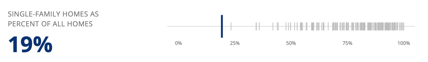
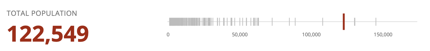
Use Brand Colors

Define Brand Colors as Variables

psc_blue <- "#15397F"
psc_red <- "#9F3515"

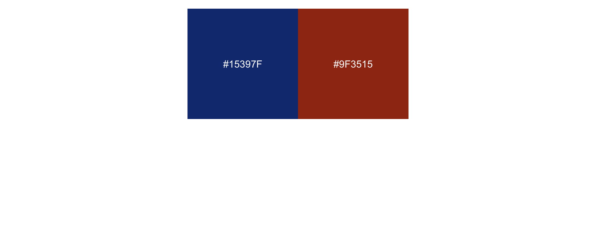
Use Brand Colors in Plots

comparison_plot <- function(
  df,
  highlight_town,
  value_type,
  highlight_color
) { }

comparison_plot <- function(
  df,
  highlight_town,
  value_type,
  highlight_color
) {
  geom_point(
    data = df |> filter(location == highlight_town),
    shape = 124,
    color = highlight_color,
    size = 10
  )
}

comparison_plot(
  df = single_family_homes,
  highlight_town = "Hartford",
  value_type = "percent",
  highlight_color = psc_blue
)

comparison_plot(
  df = total_population,
  highlight_town = "Hartford",
  value_type = "number",
  highlight_color = psc_red
)

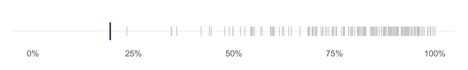
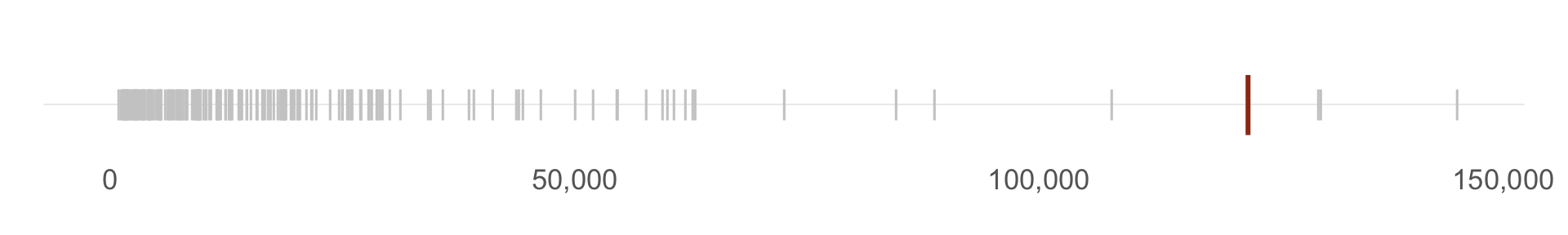
Big Numbers

big_number_plot <- function(
  value,
  text,
  value_color
) { }

big_number_plot <- function(
  value,
  text,
  value_color
) {
  ggplot() +
    # Add value
    geom_text(
      aes(
        x = 1,
        y = 1,
        label = value
      ),
      color = value_color,
      fontface = "bold",
      size = 20,
      hjust = 0
    ) +
    ...
}

big_number_plot(
  value = "19%",
  text = "Single-Family Homes as\nPercent of All Homes",
  value_color = psc_blue
)

big_number_plot(
  value = "122,549",
  text = "Total Population",
  value_color = psc_red
)

Use Brand Fonts in Plots

Make a Custom Theme

theme_psc <- function() {
  theme_void(base_family = "Open Sans") +
    theme()
}

comparison_plot(
  df = total_population,
  highlight_town = "Hartford",
  highlight_color = psc_red,
  value_type = "number"
) +
  theme_psc()

big_number_plot(
  value = "122,549",
  text = "Total Population",
  value_color = psc_red
) +
  theme_psc()

big_number_plot <- function(value, text) {
  ggplot() +
    # Add value
    geom_text(
      aes(
        x = 1,
        y = 1,
        label = value
      ),
      fontface = "bold",
      size = 20,
      hjust = 0
    ) +
    # Add text
    geom_text(
      aes(
        x = 1,
        y = 2,
        label = str_to_upper(text)
      ),
      color = "gray70",
      size = 7,
      hjust = 0
    ) +
    ...
}

big_number_plot <- function(value, text) {
  ggplot() +
    # Add value
    geom_text(
      aes(
        x = 1,
        y = 1,
        label = value
      ),
      family = "Open Sans",
      fontface = "bold",
      size = 20,
      hjust = 0
    ) +
    # Add text
    geom_text(
      aes(
        x = 1,
        y = 2,
        label = str_to_upper(text)
      ),
      family = "Open Sans",
      color = "gray70",
      size = 7,
      hjust = 0
    ) +
    ...
}

update_geom_defaults(
  geom = "text",
  aes(family = "Open Sans")
)

Tell people to do the same with a table template

---
title: "Housing Data Profiles"
format: typst
---

```{r}  
psc_blue <- "#15397F"
psc_red <- "#9F3515"
```

```{r}
update_geom_defaults()
```

```{r}
big_number_plot()
```

```{r}
comparison_plot()
```

Slides

rfor.us/posit2024slides

GitHub Repo

rfor.us/posit2024repo

Report Examples

rfor.us/consulting